Development of Surface Roughness Standards for Pathways Used by Wheelchair Users: Final Report

3. Study Findings

Literature Review

Road Roughness Measurements

The literature review found methods of measuring and recording surface profiles including the rod and level, dipstick, rolling straight-edge, profilograph (Figure 6), rolling profilers, Road-Response Type Measuring System (RRTMS) (Figure 7) and inertial profilers (Figure 8). One of the original methods was the profilograph, which was adopted in the early 1900’s, and can directly measure surface roughness by using an array of wheels on each side to establish a reference plane for measuring deviations. (Figure 6) The roughness is measured as the absolute sum of deviations of the center wheel. (Gillespie, 1992; Sayers, 1998)

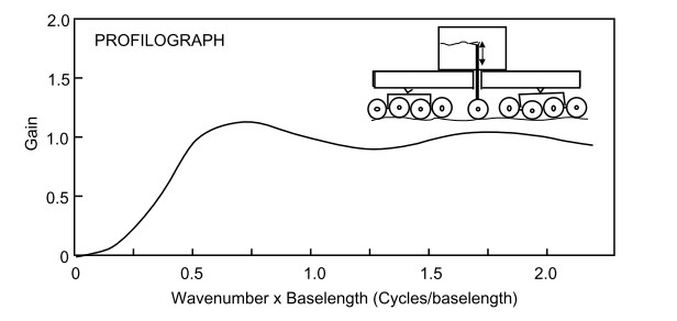
Figure 6: Schematic of Profilograph (Sayers and Karamihas 1998)

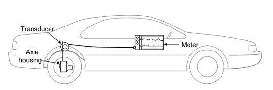
Figure 7: Schematic of RTRRMS (Sayers and Karamihas 1998)

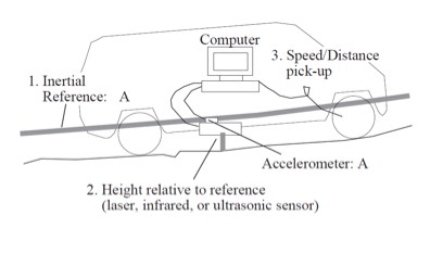
Figure 8: Schematic of Inertial Profiler (Sayers and Karamihas 1998)

During the 1960s, an automobile-mountable measurement device began a new era of surface roughness measurements, with some advantages and disadvantages. The major advantages of these systems were their low cost and their ability to mount onto any vehicle. These RTRRMS systems recorded cumulative axle displacement over a given distance and thus reported surface roughness as inches/mile. Also known as "road meters", two examples of these systems were the Mays Ride Meter and the PCA Meter. (Gillespie, 1992; Sayers, 1998)

The disadvantages to using the RTRRMS were the inconsistencies introduced by variations between the different commercialized RTRRMS systems and also that were mounted onto different automobiles that may have had different suspension systems. Consequently, measurements from identical surfaces could be different depending on which device and automobile were used. This effect was compounded by the influence of minor differences even within identical vehicles, such as fuel level, number of passengers, or tire pressure. With this variability, developing a consistent and reliable database of road roughness measures and related thresholds was impossible. The need for standardized and consistent measures was necessary throughout the world. This led to the development of an effort organized and conducted by the World Bank in Brazil in 1982 known as the International Road Roughness Experiment. One goal of the experiment was to establish a correlation and calibration standard for roughness measurements. In processing the data, it became clear that nearly all roughness measuring instruments in use throughout the world were capable of producing measures on the same scale, if that scale was suitably selected. A number of methods were tested, and the in/mi calibration reference from NCHRP Report 228 was found to be the most suitable for defining a universal scale. (Gillespie, 1992; Sayers, 1998)

Another method of measuring surface profiles is with an inertial profiler. (Figure 8) An inertial profiler uses an accelerometer and a non-contacting sensor, such as a laser transducer, to measure height. Data processing algorithms converts vertical acceleration measured by the accelerometer to an inertial reference that defines the instant height of the accelerometer in the host vehicle. The height of the reference from the ground is measured by the sensor and subtracted from the reference. The distance traveled is usually measured by wheel rotations or a speedometer. These profilers are convenient because they can be attached to any vehicle. However, because they use acceleration measurements, they are inaccurate at low speeds. Most roadway inertial profilers cannot measure accurately at speeds less than 15 km/hr. (Sayers, 1998)

The Present Serviceability Index (PSI) is another method of measuring surface roughness and performance of pavement. It is the first and most commonly used method for relative objective measures of surface condition with the public’s perception of serviceability. However, the primary use of PSI is to evaluate the ability of the pavement to serve its users by providing safe and smooth driving surfaces. Between 1958 and 1960, the American Association of State Highway Officials conducted a study of pavement performance on surfaces in Illinois, Minnesota, and Indiana. A panel of raters evaluated roadway surfaces by riding in a car over the pavement and filling out a PSR (Present Serviceability Rating) form. (Figure 9) While the PSR measurements were being conducted by the panelists, other objective measurements (Total crack length, slope variance, rutting depth, etc.) were being taken on the same roads. The PSI equation (Equation 3) was derived to be able to use the objective measurements of the road to predict the panel’s rating. These equations allowed objective measurements taken from a stretch of highway to predict the rider perception of that roadway and thus be a way to determine whether the pavement is acceptable or needs to be replaced. The PSI equations produce a scale of zero to five; five indicates an excellent ride condition while zero refers to a very poor ride quality. Manual observation is still considered possibly the strongest and most accurate evaluation of a road surface because of their attention to detail; however, it requires a substantial amount of human-hours and associated cost. (Sayers, 1998; Latif, 2009)

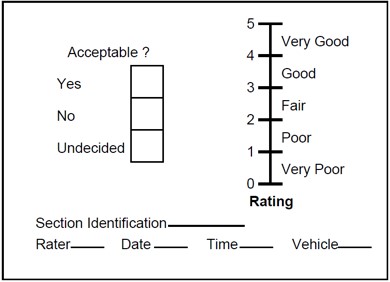
Figure 9: PSR Evaluation Form (Sayers and Karamihas 1998)

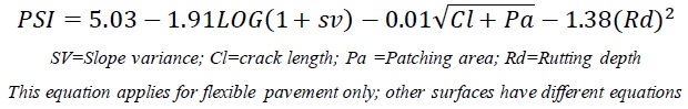
Equation 3: Present Serviceability Index

Road Roughness Analysis

The literature review also found several approaches that have been used to process the surface roughness measurements into meaningful indices. These indices include moving average, Ride Number (RN), International Roughness Index (IRI), and Power Spectral Density (PSD). However, the gold-standard for designing and evaluating roadway roughness is the (IRI) which was developed by the International Road Roughness Experiment (IRRE) and establishes equivalence between several methods of roughness measurements. The IRI also has an ASTM standard measurement protocol for consistent measurements. (ASTM E1926) The IRI is the cumulative sum of displacement of the upper mass (Ms) of a standardized ‘quarter-car’ model when it is simulated to travel over a road profile (Z(x)) which was either measured, or generated for the purposes of designing a new roadway. The characteristics of the ‘quarter-car model are shown in Figure 10 (Sayers, 1998; Loizos, 2008)

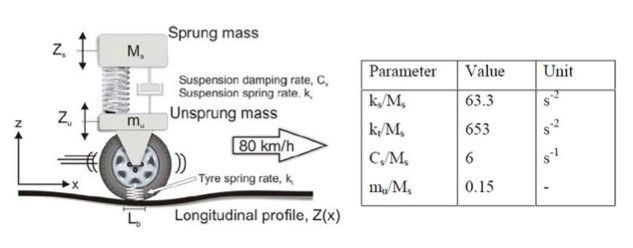
Figure 10: Quarter-car picture and variables (Loizos and Plati 2008)

The strength of the IRI is its stability and portability. Although the in/mi measure from RTRRMS has been popular since the 1940’s, as discussed above, values varied from one vehicle over time or from different vehicles on the same road. Since the IRI model is defined by its mathematical quarter-car model, it is not affected by the measurement procedure or the characteristics of the vehicle that was utilized in collecting the profile measures. Another important factor concerning the IRI is that it was designed to focus on road serviceability. Serviceability is a criterion measure for highway surfaces based on surface roughness, which is then used as a determinant need for rehabilitation of highway surfaces. (Figure 11) (Shafizadeh, 2002; Loizos, 2008)

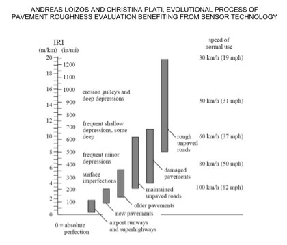
Figure 11: IRI Scale (Sayers and Karamihas 1998)

A study done in Japan addressed the usability of IRI on sidewalks used by WC’s. (Yamanaka, 2006) The study had ten subjects ride in a manual WC over nineteen different surfaces. The subjects were then asked to rate the smoothness of the ride and if they felt shaking. Vibration measurements were also recorded during the trials using speedometers attached to a caster wheel of the chair. Profile measurements were taken using a profilograph that could measure displacement on a 10mm interval. The results showed that there was a strong relationship between user assessment and vibration data. However, the relationship between the IRI and user assessment was not significant. The researchers concluded that this was probably due to the fact that the front tires of the WC would produce vibrations while running over small cracks and bumps that the profilograph, with a 10mm interval, could miss. Therefore the person would feel the bump, but the profilograph would not record it.

Although the IRI is accepted as a measure of serviceability in numerous countries, research has indicated that IRI may be limited in predicting serviceability because it is a broad measure of roughness and filters out potentially informative data from small areas of the roadway. Another analysis technique widely used to evaluate roughness is a Power Spectral Density (PSD) analysis of the road profiles.

The PSD provides a concise description of road roughness measured in frequencies and accompanying amplitudes. This is accomplished by describing the distribution of the pavement profile variance as a function of wavelength. The height (y) of the surface profile represents pavement roughness and is a function of spatial distance (x) along the pavement. To generate a PSD, a Fourier transform of the data is performed and scaled to show how the variance of the profile is spread over different frequencies. PSD analysis is valuable because it helps identify the source of the roughness. Short wavelengths (less than 3 m) are a result of irregularities of the top pavement layers while long wavelengths (10 m or longer) are caused by irregularities found in lower pavement layers. (Loizos, 2008)

PSD can also be evaluated in terms of roughness by plotting the PSD of elevation, PSD of slope, or vertical acceleration versus wavelength. The most commonly used are PSD of slope plots because they allow a direct view of the variance within a slope throughout a given distance of the pavement. Slope is also a more valuable parameter of pavement surface properties when wavelength is known. These plots can be used for the calculation of an index (Root Mean Square) of elevation or slope by calculating the area under the curve to evaluate pavement surface conditions. However, because they are dominated by longer wavelengths, these RMS values are not a reliable index measure of pavement surface smoothness. Additionally, these RMS indices do not consider parameters such as vehicle speed and characteristics in order to be used to evaluate ride quality. (Loizos, 2008) IRI and PSD are of limited value in predicting serviceability on short roadways, as they must have a reasonably long sample size to obtain accurate estimates; they are also not effective at pinpointing local defects.

To address these shortcomings, engineers have also analyzed profile data using Wavelet Theory (WT). This theory decomposes a signal into different frequency components and then presents each component with a resolution matched to its scale. It can detect sharp changes in magnitude of the profile as well as addressing the issue of location where irregularities and deformities occur. Therefore, the WT is able to identify the locations of surface revealing, depressions, settlement, potholes, surface heaving and humps, something that only manual labor intensive subjective procedures were previously able to measure accurately. The WT detects these problems through local analysis which reveals the aspects that the other signal analysis techniques miss (discontinuities in higher derivatives, breakdown points and trends). WT also addresses the issue of lost time information, which occurs in PSD analysis, by using short width and long width windows at high and low frequencies respectively. This gives WT an infinite set of possible basis functions and greatly reduced computation time. (Wei, Fwa et al.)

Subject Testing

Study Population

As of May, 2014, 76 subjects participated in our study; however, not all of the subjects traveled over every surface. Surfaces 7 and 9 were added after 17 subjects had already participated in the study. Some subjects withdrew from the study before completing every surface due to time constraints

In order to test many subjects at once, we tested at several sites. Subjects 1-17 were tested at the Wild Wood Hotel in Snowmass, CO during the National Disabled Veterans Winter Sports Clinic. Subjects 28-45 were tested at the Richmond Convention Center in Richmond, VA during the National Veterans Wheelchair Games. All other subjects were tested at the Human Engineering Research Laboratories and University of Pittsburgh in Pittsburgh, PA.

Demographic Questionnaire Data

Of the 76 subjects tested, 60 were males and 16 were females. The average age for participants was 49.0 ± 13.8. There were 37 manual WC users and 39 power wheel chair users. Most reported spending between 6-24 hrs/day in their chair. 43.4% of subjects were either somewhat unsatisfied or very unsatisfied with the pathways they typically travel, and damaged or warped pathways were their biggest complaint. Table 4 contains the questionnaire results stated above.

Table 4: Participant Demographics

Roughness Calculation

Using the IRI as a model, the roughness index was found by summing the vertical deviations of the surface profile for a given horizontal distance. It was noted however that the wheel and crack size had significant influences on how a chair would react to the surface. If the crack depth was deep enough, the wheel would be suspended by the two sides of the surface and never hit the bottom as shown in Figure 122 {sic}. Therefore, if the depth of the cracks were doubled, the chair would have the exact same reaction to the surface. The diameter and flexibility of the wheel also will determine how far down into the gap the wheel will travel. For example, a 26in diameter hard rubber tire that may be on the rear axle of the WC will not drop into a crack as far as a 2.5in diameter wheel that may be on the front of a manual WC. Because of the multitude of tires available for WCs, it was decided to choose a "standard wheel" for the analysis. The one selected for analysis was considered the worst case tire; a 2.5 in diameter hard rubber wheel (which is often used as a front caster for manual WCs).

The laser data were filtered using a 3-point moving average filter to minimize the vertical deviations caused by the noise of the laser. A "wheelpath" algorithm was then run to determine how the "standard wheel" would travel over each surface profile. The Pathway Roughness Index was calculated by summing the vertical deviations of the wheelpath data. (Figure 133) {sic}

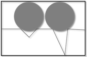
Figure 12: Schematic of Crack Depth

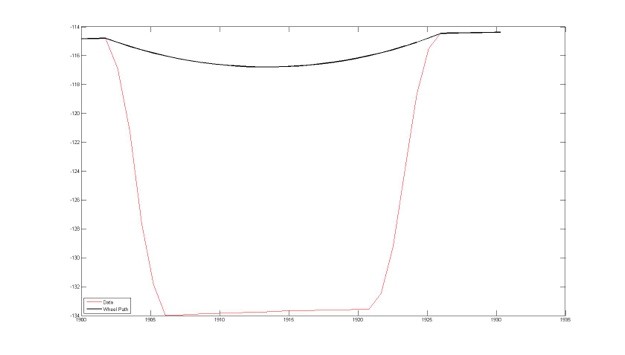
Figure 13: Picture of Wheelpath algorithm bridging a gap

The accelerations collected at the seat frame, footplates, and backrest were converted to RMS accelerations and VDV values.

Table 5 presents the average RMS accelerations and Table 6 presents the VDV values for each surface. As described earlier, ISO 2631-1 recommends using VDV instead of RMS when there are infrequent high magnitude shocks and the crest factor is greater than 9. Another way they suggest to determine which value to use is to use VDV if the following proportion is exceeded.

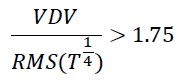
In our data analysis, this proportion was only reached at the seat accelerometer for two outside surfaces, which were both made of large concrete slabs. Because the ratio was less than 1.75 for all other surfaces, the rest of the data will only be presented as RMS accelerations.

Table 5: Average RMS Values

[Click image above to view HTML version]

Table 6: Average VDV Values

[Click image above to view HTML version]

Figure 14 is the graphical representation of the total RMS data for all surfaces based on roughness. The slopes of the linear trend lines show that as surface roughness increased, average RMS accelerations consequently increased. The slopes for the seat and footrest are similar while the slope for backrest is only about half that of the footrest. The R² values show that the data fits the linear trend line fairly well.

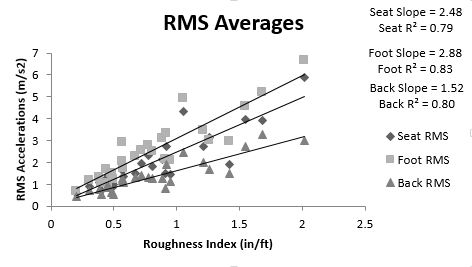
Figure 14: Total RMS Averages across all surfaces

Engineered vs. Outside

Figures 15-17 show the vibrations at the seat, footrest and backrest respectively with the engineered and outside surfaces separated. The seat values are of particular importance because vertical vibrations transferred through the seat of a seated individual are the most hazardous. The high R² values for the engineered surfaces show that vibrations for a particular surface can be predicted by knowing the surfaces roughness. The lower R² values for the outside surfaces show that there is a larger variation of data.

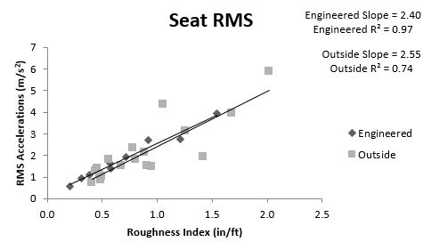
Figure 15: RMS for Seat

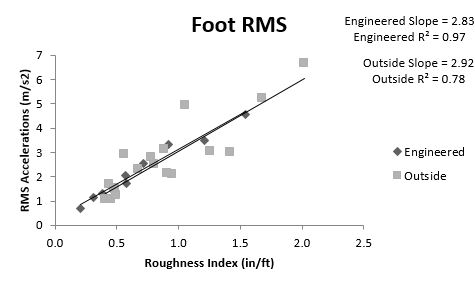
Figure 16: RMS for Footrest

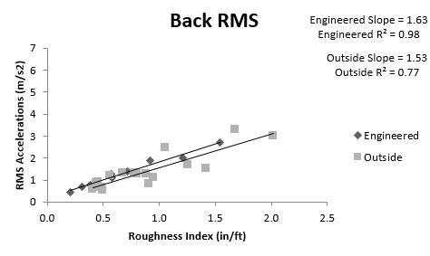
Figure 17: RMS for Backrest

Manual vs. Power (RMS Values)

Figure 18 shows the seat RMS values with manual and power WCs separated for all of the surfaces. The different slopes of the linear trend lines show that manual WCs will have a greater increase in vibrations for a particular increase in surface roughness than power WCs. The R² values suggest that the data for both types of WCs the data is fairly linear.

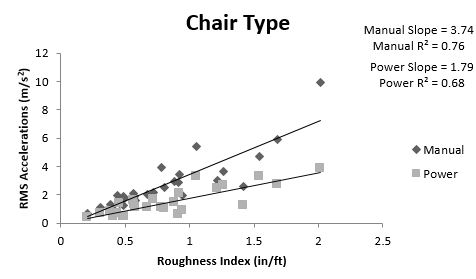
Figure 18: Seat RMS of Manual vs. Power wheelchair

The last section demonstrated that the vibration data for the engineered surfaces are much more consistent than the outside surfaces. Figure 19 displays the same axes as Figure 18 but with the engineered data only. The R² values become much higher. The manual WC trend line still has a larger slope and overall the RMS values for manual WCs are higher than power WCs. The vibration data for the roughest three surfaces show that there might be some other surface characteristic besides roughness that is contributing to the data. The vibration data from surface 8 is lower than surface 7 (especially for manual WCs) even though surface 8 is rougher according to the roughness index. The characteristics of the surfaces show that surface 8 has smaller gaps than surface 7 (1.25 inches compared to 1.55 inches), but they occur at a higher frequency (every 4 inches compared to every 8 inches). This could indicate that the size of gaps in surfaces may be more important than the frequency of the gaps. Wolf et al found a similar result in their study when they found that a brick surface with small but highly frequent bevels resulted in lower vibrations than a concrete surface that had larger gaps at large intervals (4’) between the slabs. (Wolf, 2007)

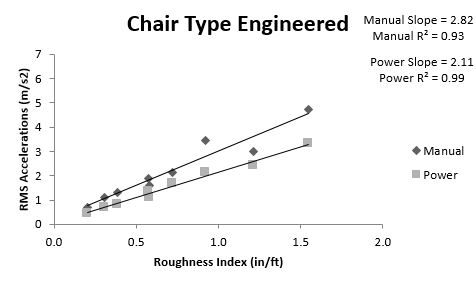
Figure 19: Seat RMS of Manual vs. Power Wheelchair Engineered

As shown in Table 5, the standard deviations of the RMS values for the engineered surfaces are roughly half the average indicating that there is large variability of data. For this reason, the majority of the data presented in this paper are presented as means without error or confidence levels. However, Figure 20 does show the average seat RMS data for all of the surfaces with 95 percent confidence bars.

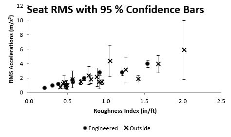
Figure 20: Seat RMS values with 95 percent confidence bars

Questionnaire Data

Table 7 displays the results from the surface questionnaire for all surfaces. Percent Acceptable is the percent of the subjects that answered that the surface was acceptable on the questionnaire. Rating mean is the average of the ratings that the subjects chose for each surface after they traveled over them. Figure 21 shows a graphical representation of the data presented in Table 7. 

Table 7: Questionnaire Results

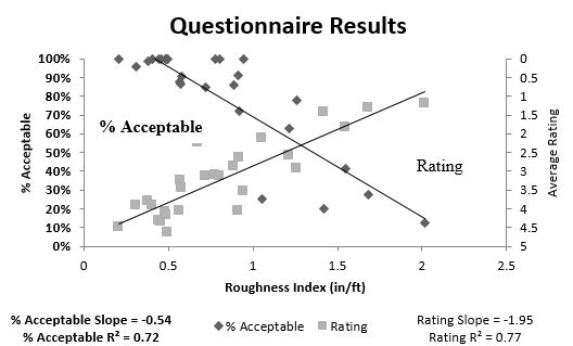
Figure 21: Questionnaire for All Surfaces  

Engineered vs. Outside (Questionnaire Results)

Tables 8 and 9 and Figures 22 and 23 show the questionnaire results broken down by engineered and outdoor surfaces. The slopes of the linear trend lines for the engineered and outside surfaces are similar for both the Percent Acceptable and Rating data. However, just like with the RMS acceleration data, there is much more variability in the outside data than the engineered data as shown by the R² values in both graphs.

Table 8: Engineered Questionnaire Results

 Table 9: Outdoor Questionnaire Results

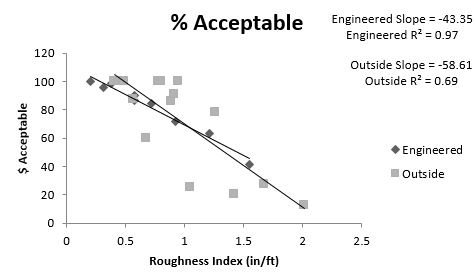
Figure 22: Percent Acceptable Engineered vs. Outside

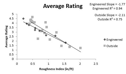
Figure 23: Average Rating Engineered vs. Outside

Manual vs. Power (Questionnaire Data)

Figures 24 and 25 show the results of the questionnaire data separated by manual and power WCs. It should be noted that even though manual WC users had higher vibrations for all engineered surfaces, on average they rated all surfaces better than power chair users.

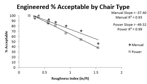
Figure 24: Percent Acceptable Manual vs. Power Wheelchair Engineered

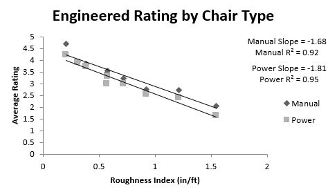
Figure 25: Rating Manual vs. Power Wheelchair Engineered