Visual Detection of Detectable Warning Materials by Pedestrians with Visual Impairments - Final Report
2 Results
2.1 Participants’ Vision
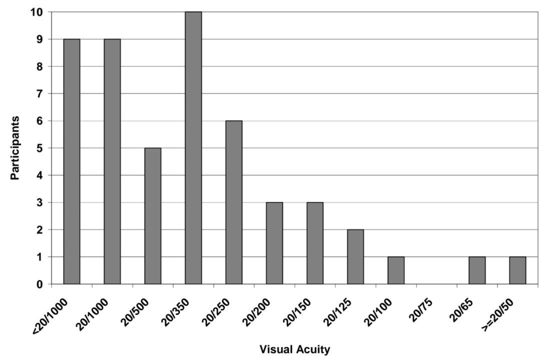
The distribution of acuity scores for participants in this study is shown in Figure 5. Normal visual acuity on this scale is 20/20, which is not shown because it would be plotted far to the right of the distribution. From the adjusted viewing distance of 1.22 m (4 ft), one participant was able to read the bottom line of the chart (smallest letters) which indicated that her acuity was 20/50 or better. Despite having relatively good acuity, this participant was retained in the study because she reported having a large visual field loss. Forty-two of the participants had visual acuities of 20/200 or less, including nine participants who were unable to read the top line (largest letter) of the acuity chart, indicating that their visual acuity was less than 20/1000.
Figure 5. Chart. Distribution of Participants’ Visual Acuity
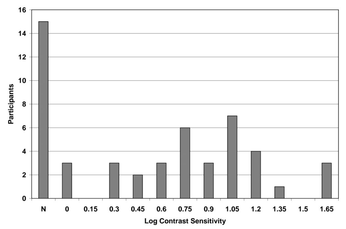
Participants’ contrast sensitivity was tested with a Pelli-Robson Contrast Sensitivity chart. The letters on this chart are all large, but the contrast of letters decreases from left to right and from the top of the chart to the bottom. Participants viewed this chart from a distance of one meter. The chart was illuminated uniformly according to the instructions provided by the manufacturer. Figure 6 shows the distribution of participants’ contrast sensitivity scores. Note that the common logarithm of contrast sensitivity is plotted along the abscissa. A log contrast sensitivity score of zero indicates that the participant was able to read only the black letters on a white background at the full level of 100 percent contrast. The nominal value for normal log contrast sensitivity is 2.0, which corresponds to the ability to distinguish letters having only 1 percent contrast. All of the participants in this study had reduced contrast sensitivity. There were 15 participants who were unable to read even the highest contrast letters on the Pelli-Robson chart from a distance of one meter. This group is shown by the “N” label on the left side of the abscissa to indicate that their contrast sensitivity was not measurable with this test.
Figure 6. Chart. Distribution of Participants’ Contrast Sensitivity Measured With the Pelli-Robson Chart
The recently revised (Fourth Edition) of the H.R.R. Pseudoisochromatic Plates test (Richmond Products, Boca Raton, FL) was used to screen participants for red-green and blue-yellow abnormalities in color vision. Because most participants in this study were not able to read any symbols on the H.R.R. Pseudoisochromatic Plates test, no results for this test are reported (see Appendix E for a description of vision testing procedures).
2.2 Lighting Conditions
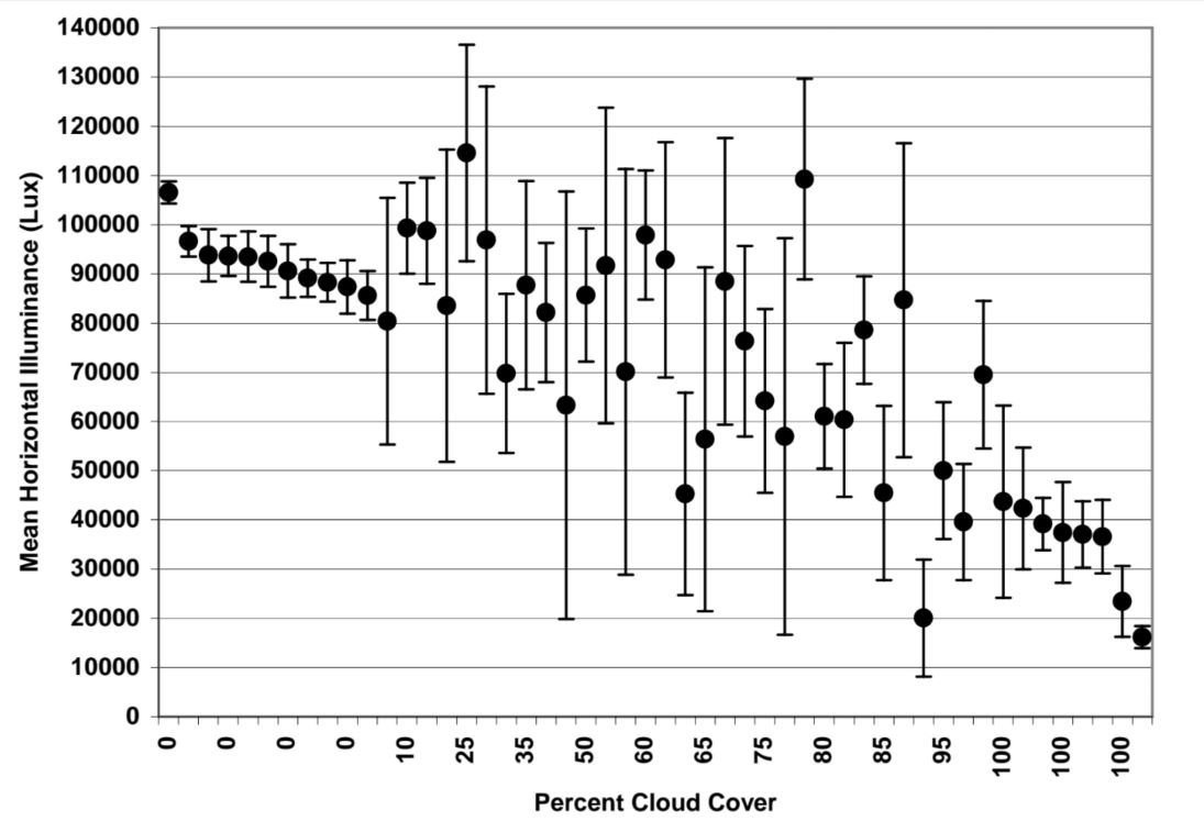
At the beginning of each testing session, experimenters visually assessed sky conditions and estimated the percent cloud cover. On each trial one measurement of horizontal illuminance was manually recorded from a Minolta T-1 Illuminance meter. The mean illuminance and standard deviation of illuminances for each participant’s trials are plotted in Figure 7. Data have been ordered from left to right by the estimated percent cloud cover that was present during the participant’s testing session. Note that the scale on the abscissa is categorical (not linear) to provide clear separation between data points. This figure shows that the fifty testing sessions varied in terms of percent cloud cover from 0 percent to 100 percent, and that mean illumination for different participants ranged from approximately 18,000 lux to 115,000 lux. Sessions with either no cloud cover (0%) or complete cloud cover (100%) tended to have low variability (smaller standard deviations) in illuminance across trials, while sessions with moderate cloud cover tended to have higher variability in horizontal illuminance across trials. As discussed below in the results section, neither illuminance level nor amount of cloud cover was significantly related to the probability of the participant seeing the detectable warning. Also, these two aspects of the lighting conditions were not significantly related to the probability of the participant giving a detectable warning a high conspicuity rating.
Figure 7. Graph. Horizontal Illuminance (Mean and Standard Deviation) for Each Participant’s Trials by the Estimated Percent Cloud Cover During the Testing Session
2.3 Visual Detection
For each sidewalk type, Table 4 shows the percentage of participants who were able to see each detectable warning at 2.44 m (8 ft) and at 7.92 m (26 ft). Although most of the detectable warnings tested in this study were seen by most participants at a distance of 2.44 m (8 ft), a few combinations of sidewalk type and detectable warning color were not seen by many participants. At greater distance, up to 7.92 m (26 ft), certain combinations of detectable warning color and sidewalk were more likely to be seen than others.
Sidewalk color had an important influence on the number of participants who could see the single-color detectable warnings. Two-color (black-and-white) detectable warnings were seen by a high percentage of participants at all distances tested on all four sidewalk colors tested.
|
Detect-able Warning Colors |
Brick | Asphalt | White | Brown | ||||
|---|---|---|---|---|---|---|---|---|
|
% seen at 8 ft |
% seen at 26 ft |
% seen at 8 ft |
% seen at 26 ft |
% seen at 8 ft |
% seen at 26 ft |
% seen at 8 ft |
% seen at 26 ft |
|
| White | 96 | 86 | 98 | 88 | 66 | 28 | 98 | 86 |
| Light Grey | 84 | 50 | 98 | 78 | 94 | 76 | 86 | 58 |
| White Concrete | 94 | 80 | 98 | 88 | 36 | 10 | 100 | 82 |
| Brown Concrete | 68 | 32 | 98 | 64 | 98 | 84 | 36 | 8 |
| Dark Grey | 84 | 64 | 78 | 46 | 100 | 86 | 92 | 68 |
| Federal Yellow | 94 | 78 | 98 | 88 | 88 | 62 | 98 | 80 |
| Pale Yellow | 96 | 74 | 98 | 88 | 82 | 58 | 98 | 76 |
| Bright Red | 84 | 62 | 92 | 66 | 100 | 86 | 94 | 68 |
| Orange-Red | 76 | 56 | 92 | 68 | 98 | 84 | 86 | 66 |
| Black | 98 | 68 | 78 | 40 | 96 | 82 | 96 | 68 |
| Black with White Border | 98 | 78 | 98 | 82 | 98 | 78 | 98 | 82 |
| Black with White Stripes | 96 | 86 | 100 | 86 | 98 | 86 | 96 | 84 |
| White with Black Border | 96 | 86 | 98 | 88 | 96 | 76 | 98 | 90 |
2.4 False Detections
On each of the white, brown, and asphalt side walks, each participant experienced two trials in which there was a flat blank panel on the sidewalk instead of a bumpy detectable warning. Out of 300 total blank trials, 11 (3.7 percent) resulted in “false alarms” or false detections where the participant reported seeing a detectable warning even though the target was a blank panel. Nearly half of the false detections were due to a single participant who reported seeing a detectable warning on 5 out of 6 of her blank trials. This participant’s results indicate that she responded appropriately to the actual detectable warnings despite the false detections on blank trials. If her data are set aside, the false alarm rate for the remaining group of 49 participants was 2 percent. The low false alarm rate is consistent with the instructions to participants to report that they could see a detectable warning when they were “confident” that there was a detectable warning on the sidewalk.
2.5 Visual Detection Distance
As described in the Method section, the maximum distance up to 7.92 m (26 ft) at which each participant could see each detectable warning was measured. These data were then analyzed at 1-foot intervals from 2.44 m (8 ft) to 7.92 m(26 ft) by counting the number of participants at each distance who were able to see the detectable warning. For this analysis, we assumed that participants who could see a particular detectable warning from a greater distance could also see it from closer distances. For example, if a participant first saw the detectable warning from a maximum distance of 4.3 m (14 feet), and saw the detectable warning when tested at the 2.44 m (8 ft) distance, then we assumed that the participant could also see the detectable warning at all intermediate distances between 2.44 m (8 ft) and 4.3 m (14 ft).
The results of this analysis are summarized in Figure 8 through Figure 20. In each of these figures, the percentage of participants (n = 50) who were able to see a particular detectable warning from distances between 2.44 m (8 ft) and 7.92 m (26 ft) is plotted at 1-foot intervals. For clarity of presentation, four different lines, corresponding to the four different sidewalk colors tested have been drawn to connect the data points. These lines show how the percentage of participants who were able to see the detectable warning changes with distance for the four different sidewalk colors tested. For any observed percentage value (P) plotted in Figure 8 through Figure 20, a 95-percent confidence interval for the true population percentage ma y be constructed by applying the formula:
95% confidence interval = [P-1.96 (SQRT(P*(1-P)/50), P+1.96 (SQRT(P*(1-P)/50)].
For the reader’s convenience, confidence intervals for several values of P are given in Table 5, however, to assure clarity of presentation, no confidence bounds are shown in Figures 8 through Figure 20.
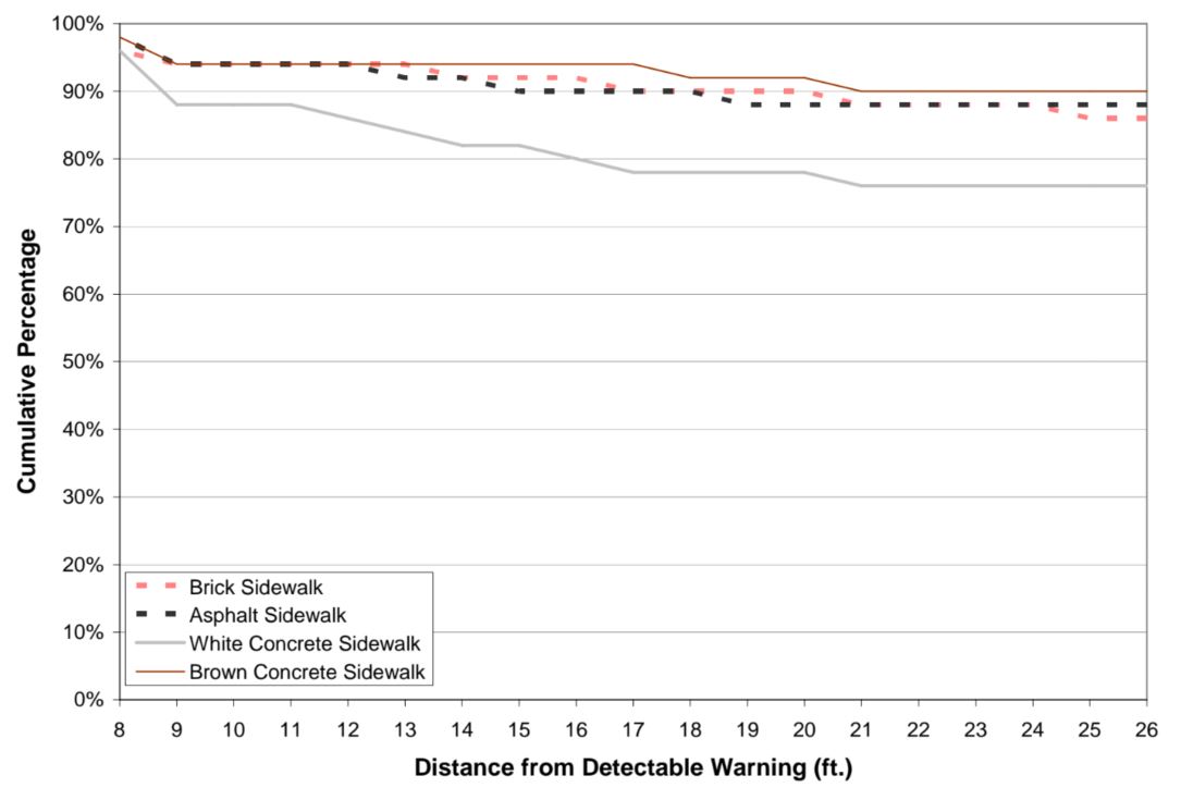
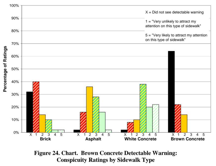
As expected, the percentage of participants who were able to see the detectable warning increases with distance from 7.92 m (26 ft) to 2.44 m (8 ft). Some of the detectable warning colors tested had much higher rates of visual detection at both 2.44 m (8 ft) and at 7.92 m (26 ft) than other colors. In cases where the sidewalk color is similar to the detectable warning color, the percentage of participants who were able to see the detectable warning is reduced. In fact, the least detectable combinations were the white “concrete” detectable warning on the white sidewalk and the brown “concrete” detectable warning on the brown sidewalk. In these cases, the detectable warning color and the sidewalk color were nearly identical.
| Percentage | Lower bound | Upper bound |
|---|---|---|
| 5% | 0% | 11% |
| 10% | 2% | 18% |
| 15% | 5% | 25% |
| 20% | 9% | 31% |
| 25% | 13% | 37% |
| 30% | 17% | 43% |
| 35% | 22% | 48% |
| 40% | 26% | 54% |
| 45% | 31% | 59% |
| 50% | 36% | 64% |
| 55% | 41% | 69% |
| 60% | 46% | 74% |
| 65% | 52% | 78% |
| 70% | 57% | 83% |
| 75% | 63% | 87% |
| 80% | 69% | 91% |
| 85% | 75% | 95% |
| 90% | 82% | 98% |
| 95% | 89% | 100% |
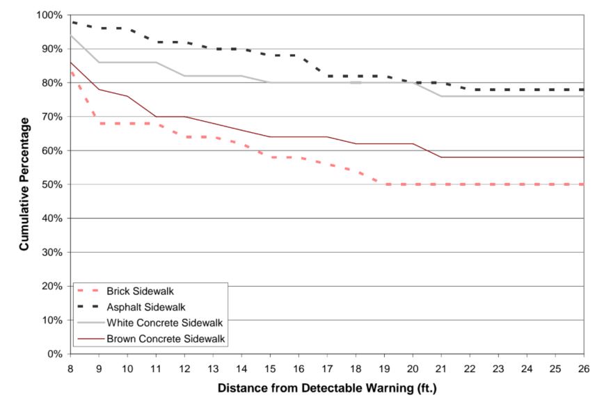
Detection distances for the 10 single-color detectable warnings are shown in Figure 8 through Figure 17. In these 10 figures, the 4 plotted lines tend to spread apart, indicating that the percentage of participants who can see these detectable warnings depends on the sidewalk type. However, in Figure 18 through Figure 20, which show data for the black-and-white patterned detectable warnings, the four plotted lines tend to run close together, indicating that the percentage of participants who were able to see these black-and-white patterned detectable warnings does not depend strongly on sidewalk type. Overall, the black-and-white patterned detectable warnings tended to be seen by more participants than most of the single color detectable warnings.
Figure 8. Graph. White Detectable Warning: Percentage of Participants Who Could See the Detectable Warning at Each Distance
Figure 9. Graph. Light Gray Detectable Warning: Percentage of Participants Who Could See The Detectable Warning at Each Distance
Sidewalk Figure 10. Graph. White Concrete Detectable Warning: Percentage of Participants Who Could See the Detectable Warning at Each Distance
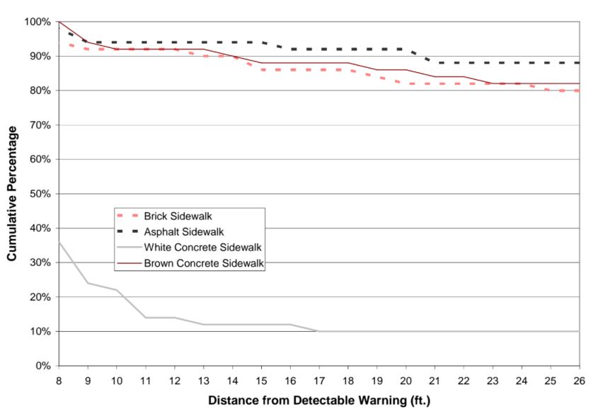
Figure 11. Graph. Brown Concrete Detectable Warning: Percentage of Participants Who Could See the Detectable Warning at Each Distance
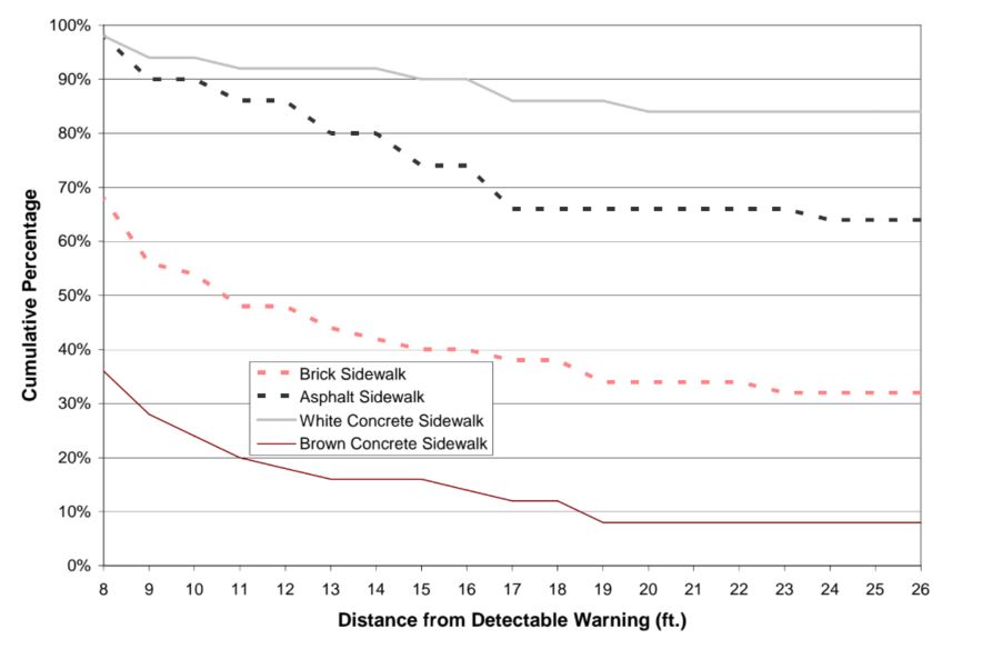
Figure 12. Graph. Dark Gray Detectable Warning: Percentage of Participants Who Could See the Detectable Warning at Each Distance
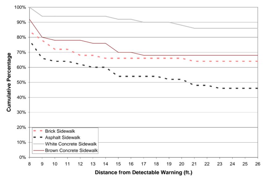
Figure 13. Graph. Federal Yellow Detectable Warning: Percentage of Participants Who Could See the Detectable Warning at Each Distance
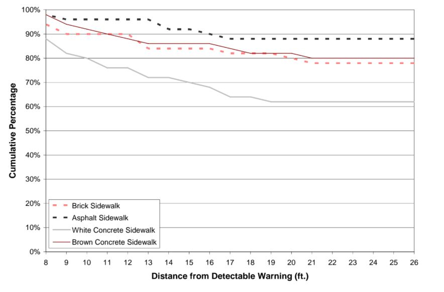
Figure 14. Graph. Pale Yellow Detectable Warning: Percentage of Participants Who Could See the Detectable Warning at Each Distance
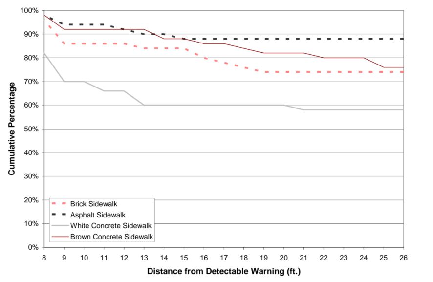
Figure 15. Graph. Bright Red Detectable Warning: Percentage of Participants Who Could See the Detectable Warning at Each Distance
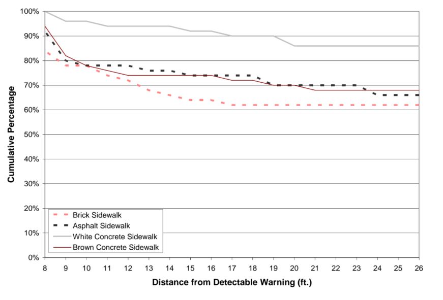
Figure 16. Graph. Orange-Red Detectable Warning: Percentage of Participants Who Could See The Detectable Warning at Each Distance
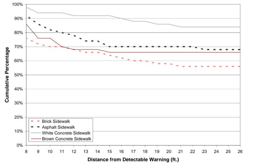
Figure 17. Graph. Black Detectable Warning: Percentage of Participants Who Could See the Detectable Warning at Each Distance
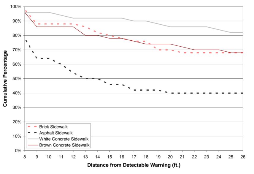
Figure 18. Graph. Black with White Border Detectable Warning: Percentage of Participants Who Could See the Detectable Warning at Each Distance
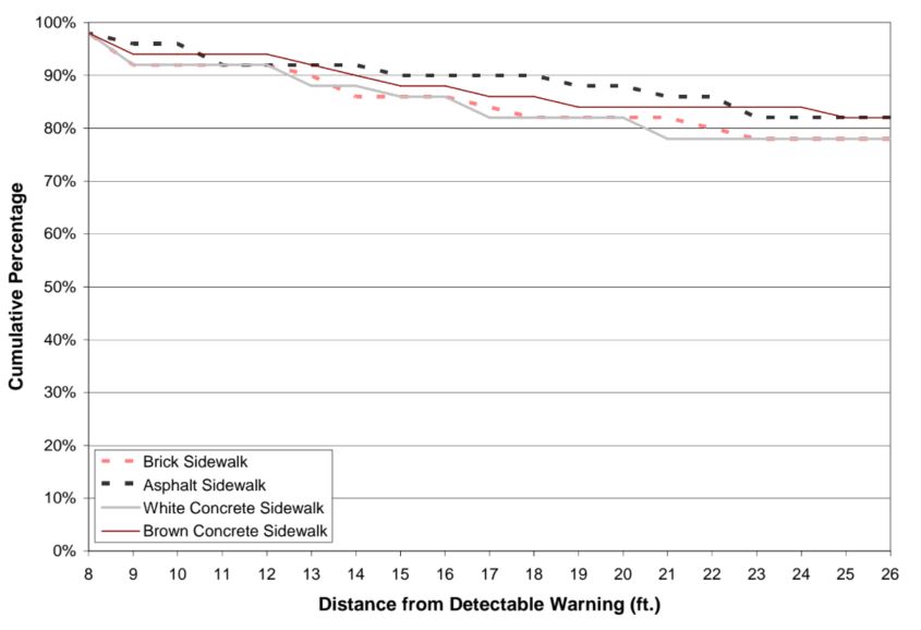
Figure 19. Graph. Black-and-White Stripes Detectable Warning: Percentage of Participants Who Could See the Detectable Warning at Each Distance
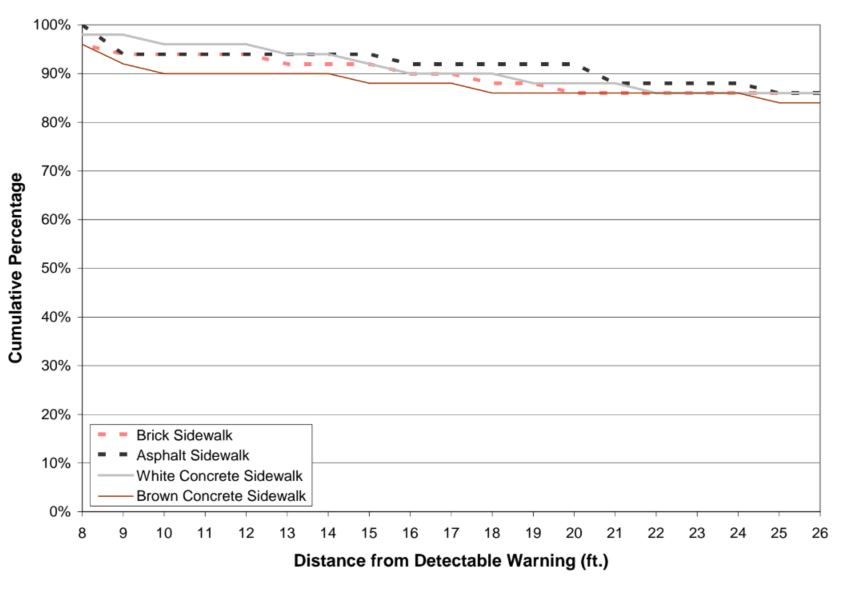
Figure 20. Graph. White with Black Border Detectable Warning: Percentage of Participants Who Could See the Detectable Warning at Each Distance
2.5.1 Comparing Visual Detection Distances for Detectable Warnings
For practical purposes, someone trying to decide between two or more available detectable warning colors for a particular sidewalk application may want to know which of the colors could be seen by people with visual impairments from the greatest distance. As shown by the previous set of figures, visual detection depends on the color of the sidewalk as well as the color of the detectable warning. Thus, for a given sidewalk type, it is necessary both to know which of the detectable warning colors tested in this study could be seen at greater distances than other colors and to have a means to decide whether any observed differences in detection distance were statistically significant.
The data on maximum visual detection distance were constrained by the experimental procedure which permitted minimum and maximum viewing distances of 2.44 m (8 ft) and 7.92 m (26 ft). The data are strongly skewed, with many trials resulting in visual detection at a distance of 7.92 m (26 ft). Other trials resulted in detection at various distances between 2.44 m (8 ft) and 7.92 m (26 ft), and some trials did not result in detections. Although viewing distances closer than 2.44 m (8 ft) were not tested, the study team coded detection distance for trials with non-detections as zero feet. In order to compare the detection distances for the 13 detectable warnings, we performed a series of pairwise comparisons using a non-parametric statistic appropriate for repeated measures data. Using SAS statistical software, we computed the Wilcoxon Signed-Rank statistic for each of the 78 possible pairwise comparisons of the 13 detectable warnings on a given sidewalk. In order to control the probability of the statistical Type I error at .05 across the entire set of 78 comparisons, we used a criterion of α = .05 / 78 = .000641 for each pairwise comparison. This method for controlling Type I error is conservative. It controls the probability of claiming statistically significant differences between detectable warnings where no differences actually exist, however, this method may risk obscuring some interesting, and potentially real practical differences observed in this study. Therefore, in addition to reporting statistically significant differences in the conservative manner described above, we have also reported the direction of pairwise differences which would have been considered statistically significant if the two detectable warnings had been tested in isolation, rather than as part of a set of multiple comparisons. Thus, for this second less conservative statistical decision criterion we set a criterion of α = .05 for each pairwise comparison.
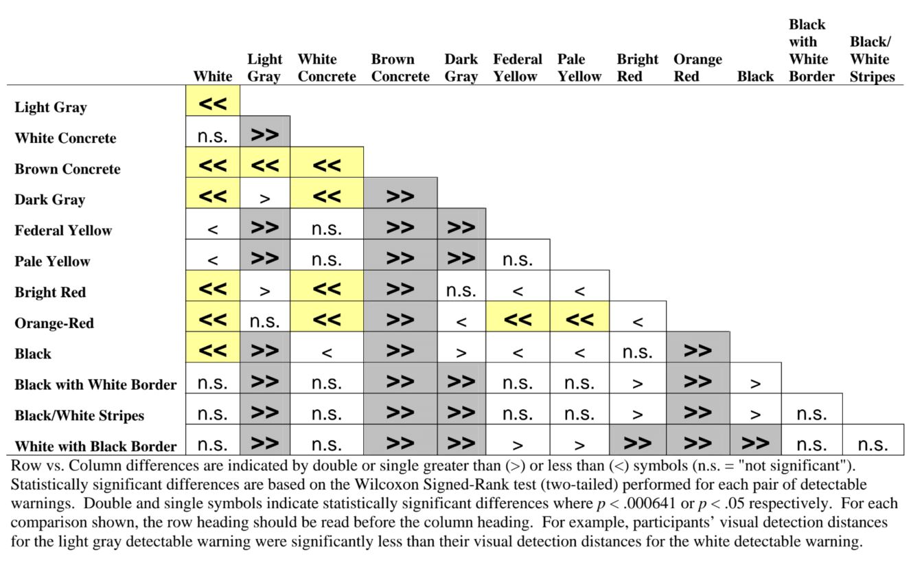
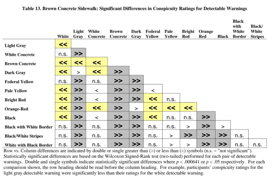
The results of the analyses are summarized in Table 6 through Table 9. Each of these tables corresponds with one of the four sidewalk types tested. The row and column headings refer to the detectable warning colors tested. The results of the pairwise comparison between detectable warnings listed in rows and those listed in columns are shown at the intersection of the appropriate row and column. The double “greater than” symbol (>>) indicates that the detectable warning color heading the row was seen from a significantly greater distance than the detectable warning color heading the column based on the conservative criterion where (p < .000641). The single “greater than” symbol (>) indicates that the detectable warning color heading the row was seen from a significantly greater distance than the detectable warning color heading the column based on the less conservative criterion where (p < .05). Similarly, the double “less than” symbol (<<) and single “less than” symbol (<) indicate that the detectable warning color heading the row was seen from significantly less distance than the detectable warning color heading the column based on the two criteria described above. The notation “n.s.” indicates that observed differences in detection distance were not statistically significant (p > = .05). For example, on the brick sidewalk the three black -and -white patterned detectable warnings were not significantly different from each other in terms of detection distance. Note that none of the significant differences designated by a single “greater than” or single “less than” symbol is statistically significant by the more conservative criterion.
The interaction between detectable warning color and sidewalk color is apparent from comparing the pattern of results across the four sidewalk types (Table 6 through Table 9). There are several cases where one detectable warning color may be seen from a greater distance than a second detectable warning color on a particular sidewalk type, but for a different sidewalk type, the second detectable warning color may be seen from a greater distance than the first. For example, the federal yellow detectable warning is seen from significantly greater distances than the dark gray detectable warning on all sidewalk types except for the white sidewalk, where the dark gray is seen from significantly greater distances than the federal yellow.
Table 6. Brick Sidewalk: Significant Differences in Visual Detection Distance for Detectable Warnings
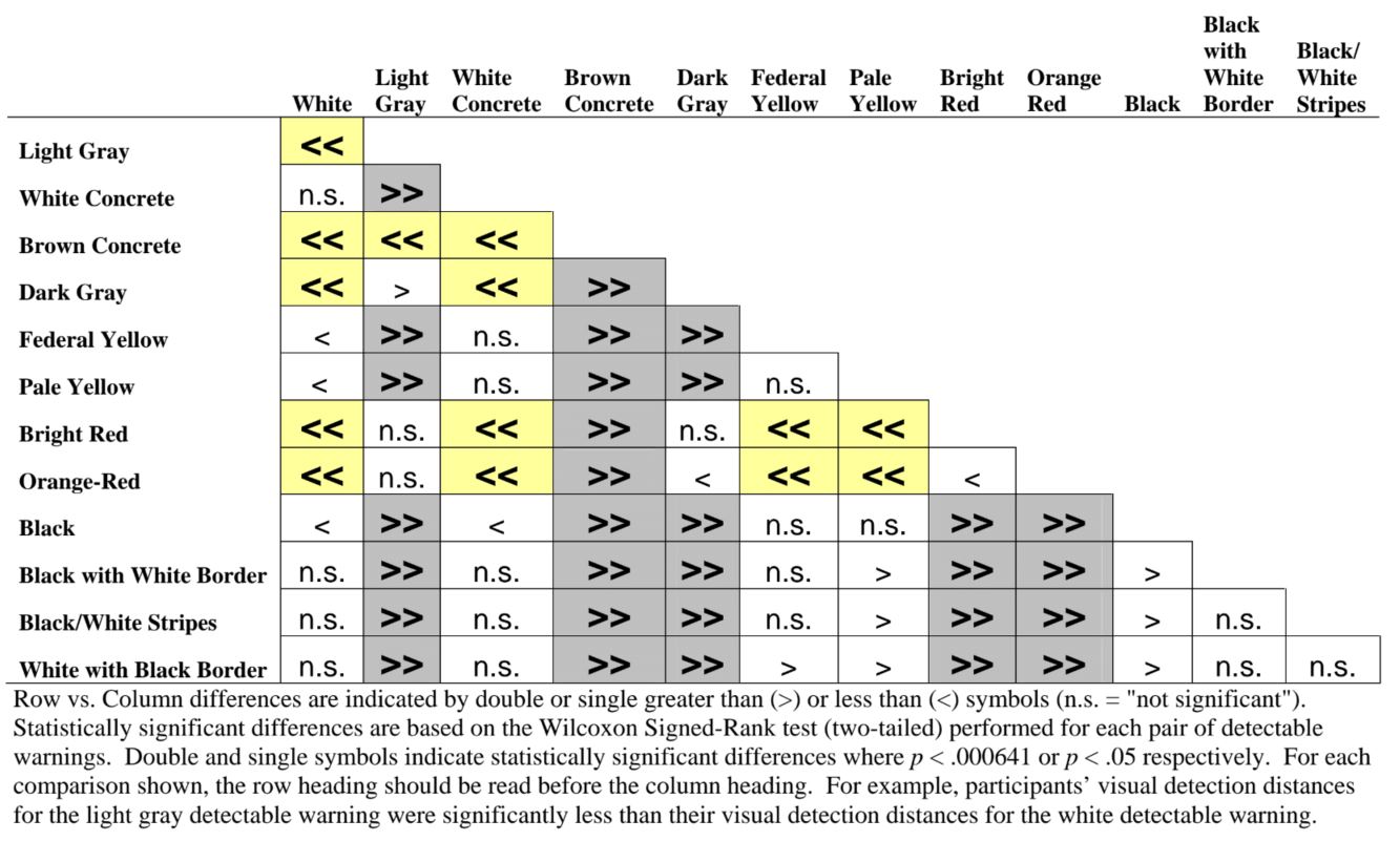
Table 7. Asphalt Sidewalk: Significant Differences in Visual Detection Distance for Detectable Warnings
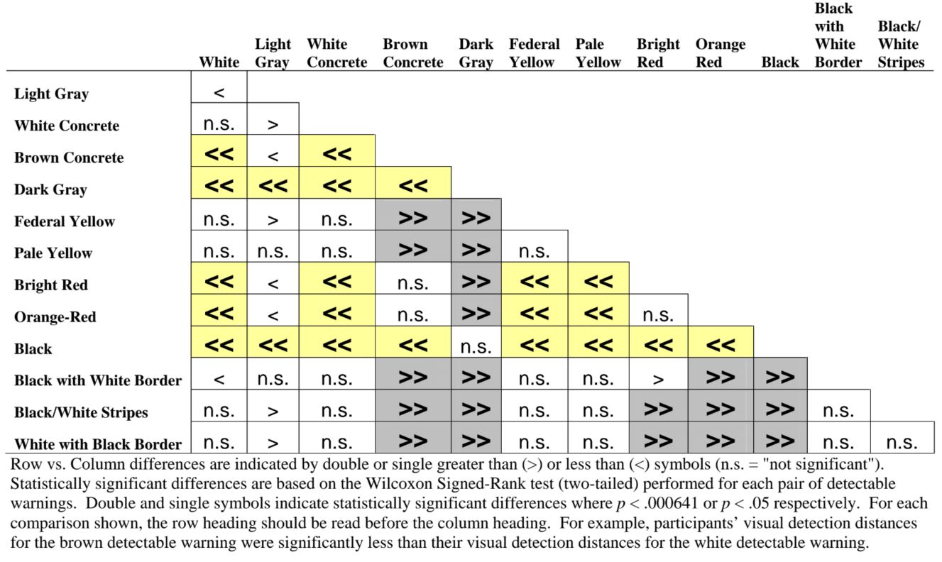
Table 8. White Concrete Sidewalk: Significant Differences in Visual Detection Distance for Detectable Warnings
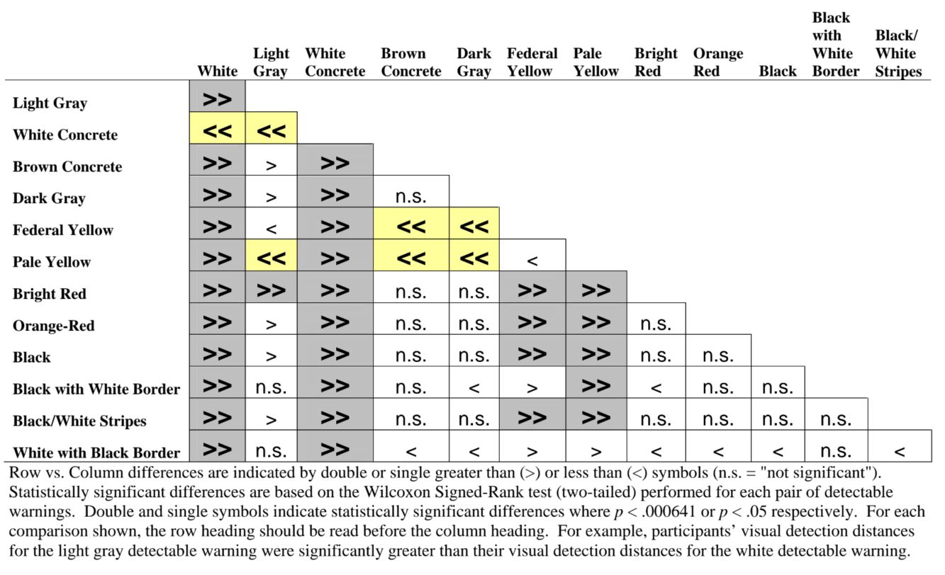
Table 9. Brown Concrete Sidewalk: Significant Differences in Visual Detection Distance for Detectable Warnings
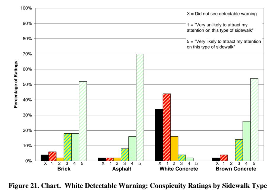
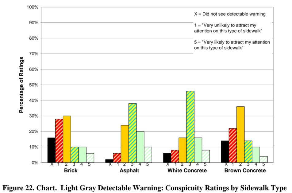
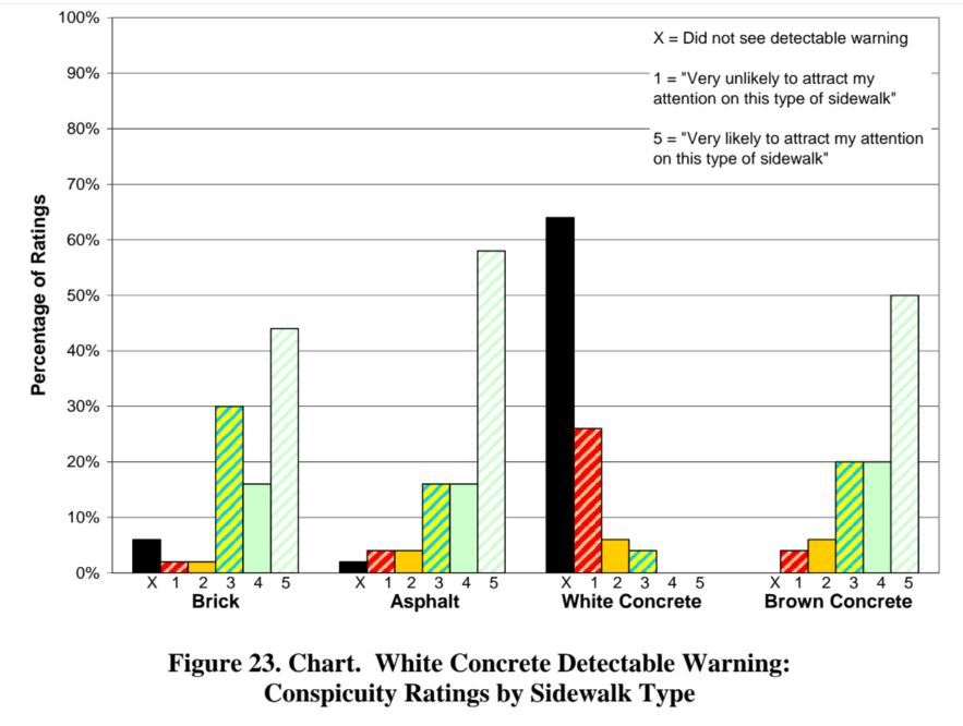
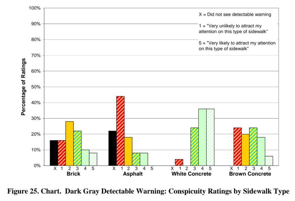
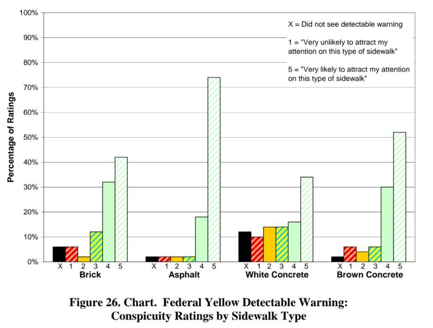
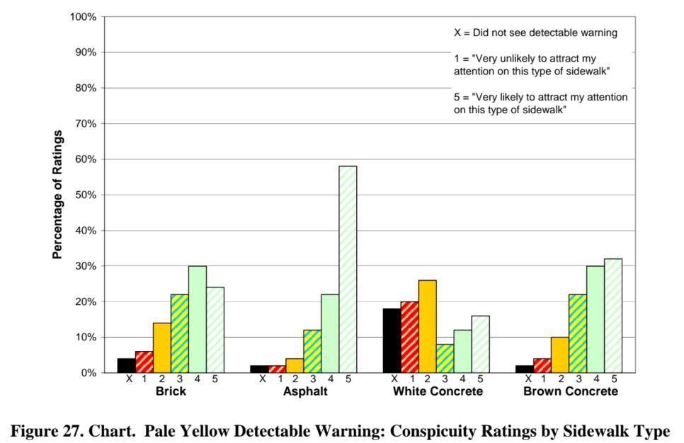
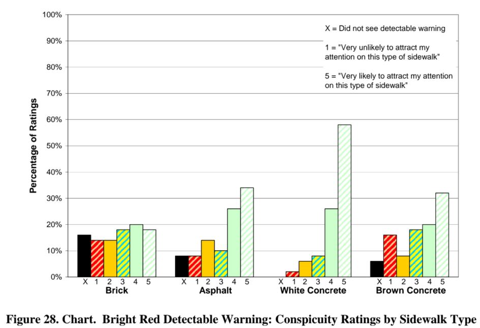
2.6 Conspicuity Ratings
Participants rated the conspicuity of each detectable warning that they could see on a numerical scale that ranged from 1 (very unlikely to attract my attention on this type of sidewalk) to 5 (very likely to attract my attention on this type of sidewalk). A rating of zero (or “X” in the figures below) was assigned by the experimenter to those detectable warnings that were not detected from the viewing distance of 2.44 m (8 ft). Figure 21 through Figure 33 show the distributions of conspicuity ratings provided by participants. Each figure includes four separate distributions and represents all 50 participants’ responses to a single detectable warning on one of the four sidewalk types. Thus, for each sidewalk, the sum of the heights of the bars is 100 percent. Distributions with many responses in the 4 or 5 categories indicate high conspicuity ratings and distributions, while many responses in categories X, 1, and 2 indicate low conspicuity ratings or an inability to see the detectable warning at all. Results for most detectable warnings varied between the different sidewalks. However, the three black-and-white patterned detectable warnings received consistently high conspicuity ratings on all four sidewalks.
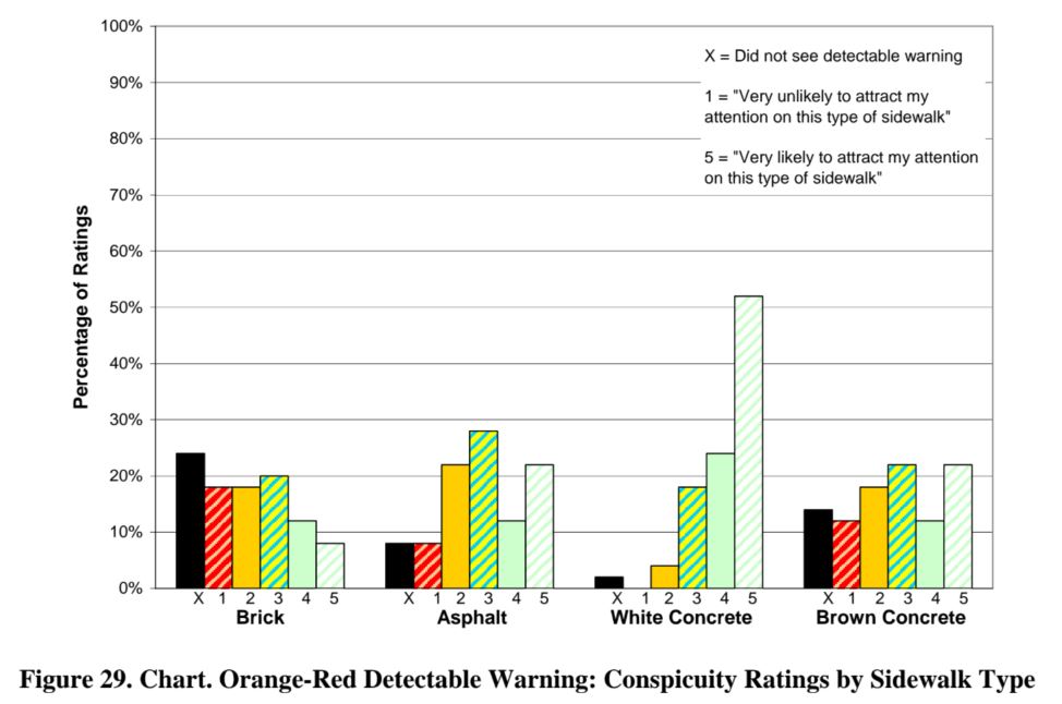
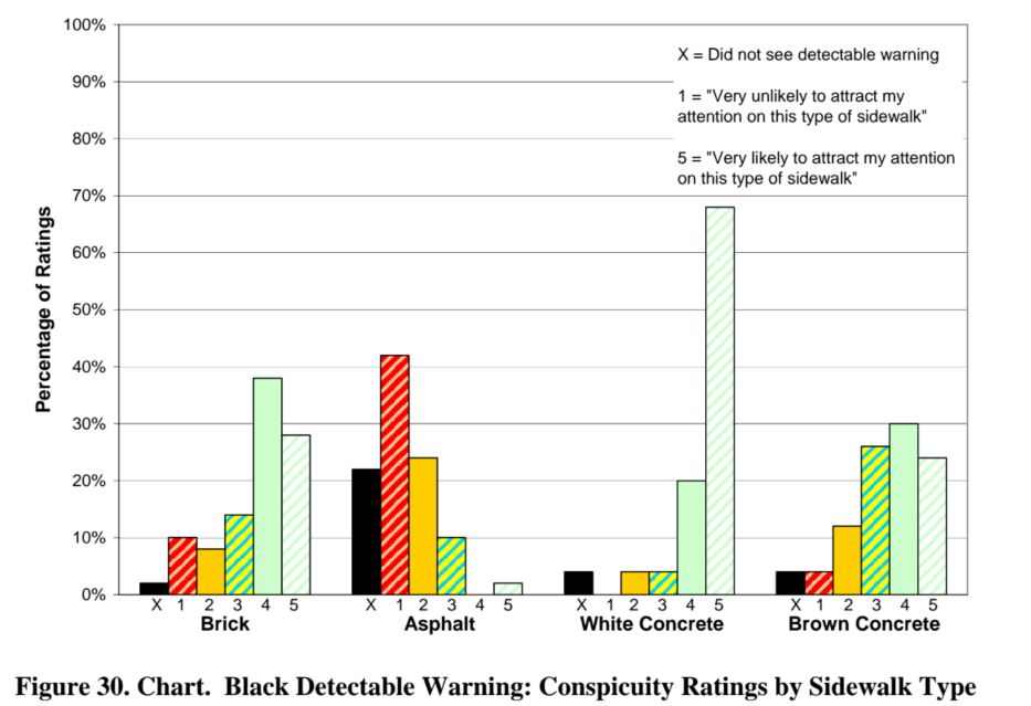
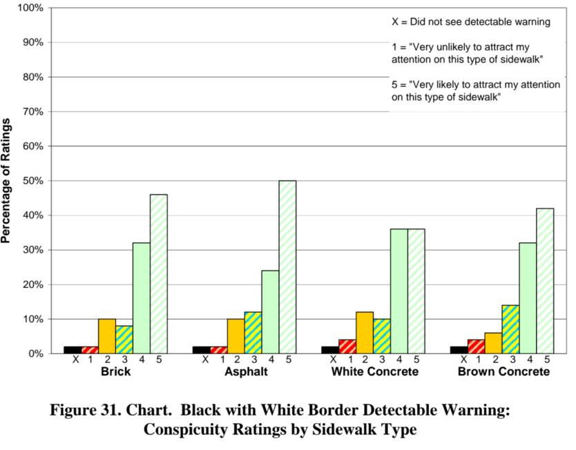
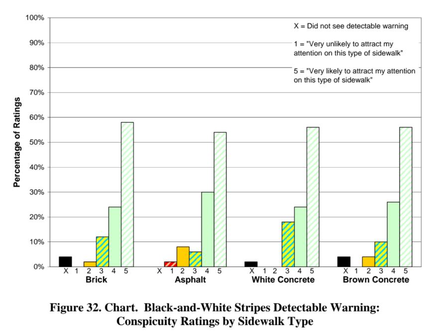
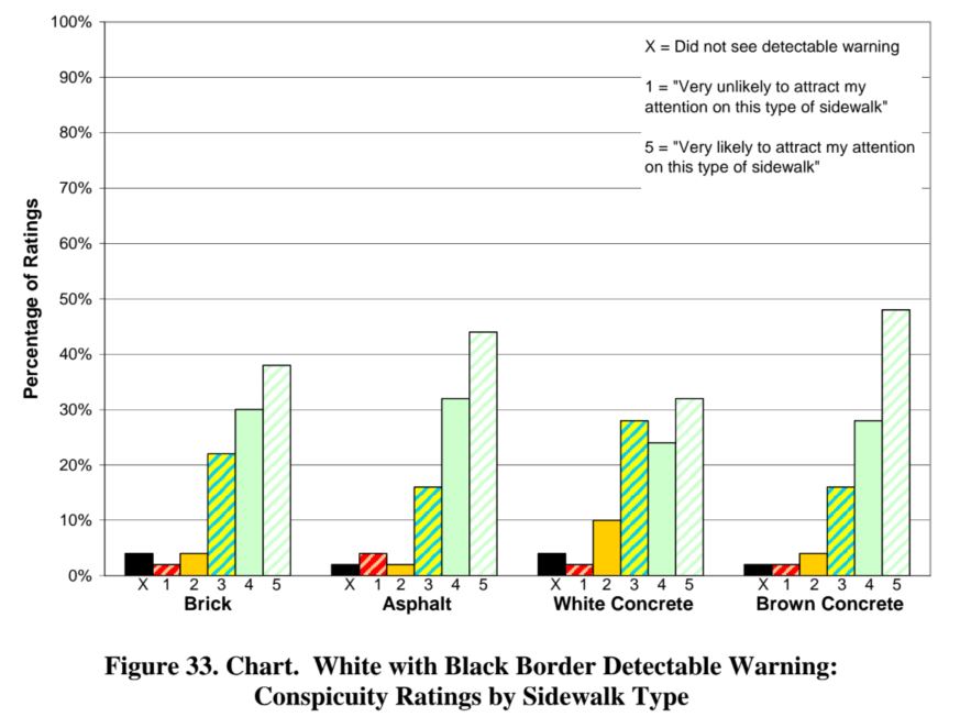
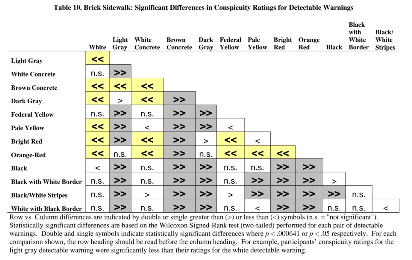
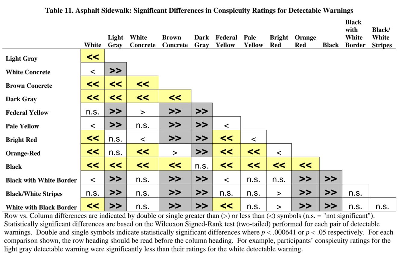
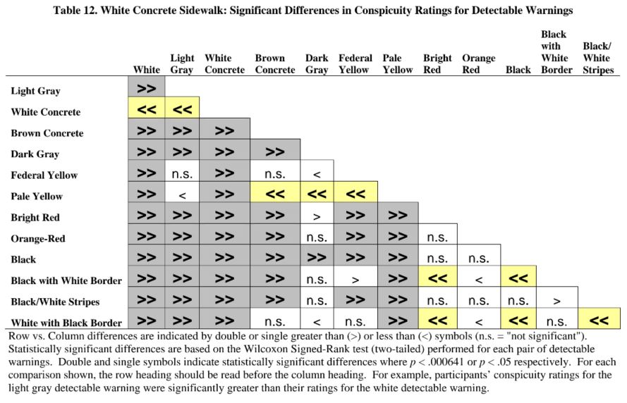
We compared conspicuity ratings for the set of detectable warnings using the same non-parametric statistical procedure that we used to compare detection distances (described in Section 2.5.1). The results of these analyses are summarized in Table 10 through Table 13. Each of these figures corresponds to one of the four sidewalk types tested. The row and column headings refer to the detectable warning colors tested. The results of the pairwise comparisons between detectable warnings listed in rows and those listed in columns are shown at the intersection of the appropriate row and column. The double “greater than” symbol (>>) indicates that the detectable warning color heading the row was rated significantly higher in conspicuity than the detectable warning color heading the column based on a conservative criterion where (p < .000641). The single “greater than” symbol (>) indicates that the detectable warning color heading the row received significantly greater conspicuity ratings than the detectable warning color heading the column based on a less conservative criterion where (p < .05). Similarly, the double “less than” symbol (<<) and single “less than” symbol (<) indicate that the detectable warning color heading the row received significantly lower conspicuity ratings than the detectable warning color heading the column based on the two statistical criteria described above. The notation “n.s.” indicates that observed differences in conspicuity ratings were not statistically significant (p > = .05).
The patterns of statistically significant differences for conspicuity ratings shown in Table 10 through Table 13 are similar, but not identical, to the patterns of statistically significant differences for detection distances shown in Table 6 through Table 9. As expected, detectable warnings that are more conspicuous are generally seen from greater distances. In some cases, two detectable warnings that do not differ significantly in detection distance on a particular sidewalk may differ significantly in conspicuity ratings on that sidewalk. In other cases, two detectable warnings that do not differ significantly in conspicuity ratings may differ significantly in detection distance.
For conspicuity ratings, 202 of the 312 pairwise comparisons summarized in Table 10 through Table 13 revealed statistically significant differences with the conservative decision criterion (p < .000641) and an additional 60 statistically significant differences are revealed by the less conservative criterion (p < .05). For the visual detection distance measure, only 164 of the 312 pairwise comparisons summarized in Table 6 through Table 9 revealed statistically significant differences (p < .000641) with an additional 42 significant differences revealed by the less conservative criterion (p < .05). These results suggest that in the present study conspicuity ratings were a more sensitive measure than visual detection distance for evaluating the visibility of detectable warnings. However, it is possible that the detection distance measure would have been more sensitive if viewing distances greater than 7.92 m (26 ft) (and less than 2.44 m (8 ft)) were included in the experimental protocol.
2.7 Comparing Visual Detection Rates and High Conspicuity Ratings for Detectable Warnings
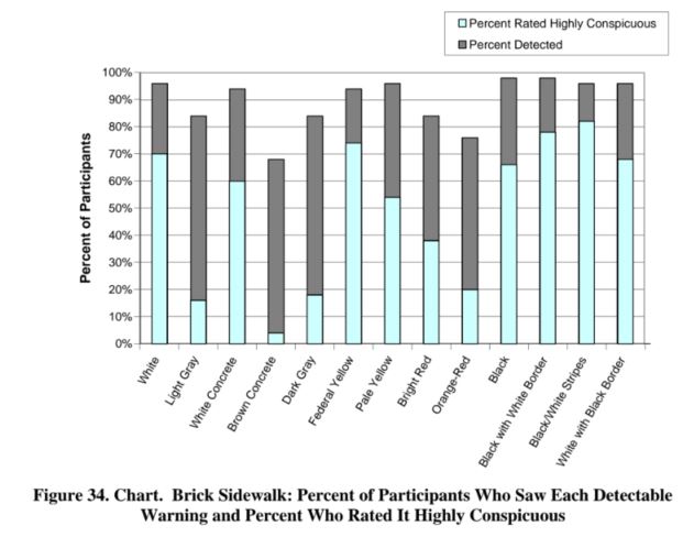
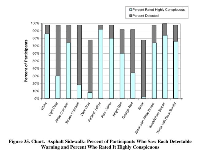
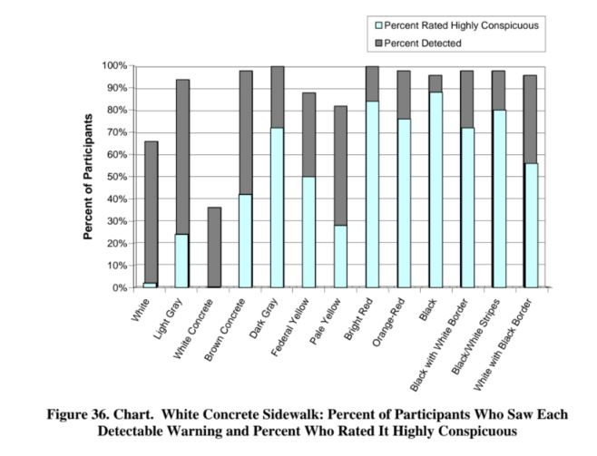
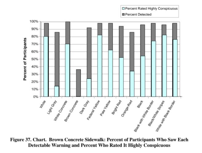
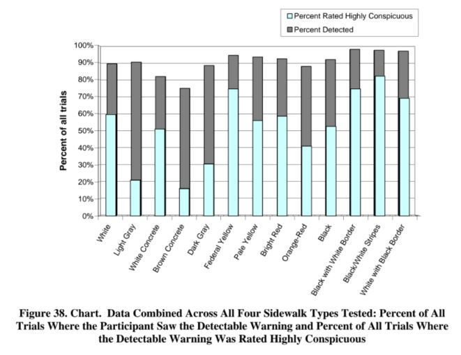
The percentages of participants giving high conspicuity ratings for each detectable warning by sidewalk combination are shown in Table 14. These data, together with data on percentages of participants who saw each detectable warning (from Table 4) are compared in Figure 34 through Figure 38.
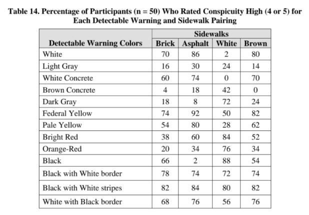
Figure 34 through Figure 37 show the percentage of participants who were able to see each detectable warning from 2.44 m (8 ft) and the percentage of participants who rated the detectable warning as having high conspicuity (giving a rating of 4 or 5). Figure 38 shows the data combined across all participants and all trials for the four sidewalk types. To the extent that the sample of participants in this study is representative of pedestrians with visual impairments, the data shown in Figure 34 through Figure 37 may be used to choose detectable warning colors that are most likely to be highly visually detectable for a particular sidewalk type. Note that when detectable warning color was similar to the side walk color, the number of people who would be served by the visual properties of the detectable warning decreased markedly. The black-and-white stripe pattern was seen by nearly all participants and was highly conspicuous on all four sidewalks tested.
2.8 Effects of Luminance Contrast on Visual Detection and Conspicuity of Detectable Warnings
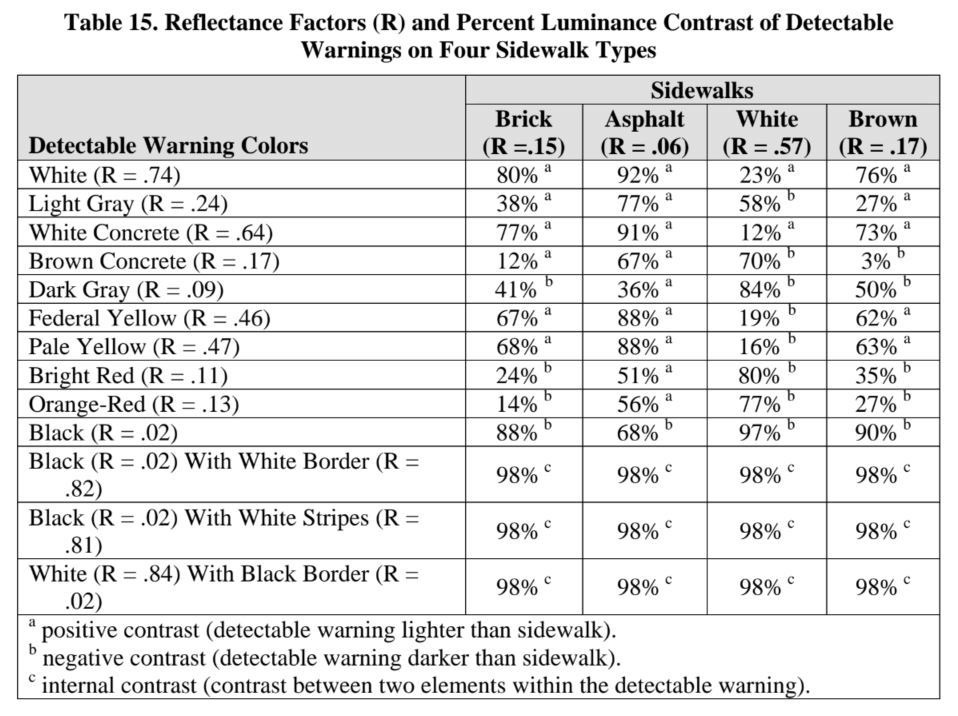
Reflectance factors for each detectable warning and sidewalk were measured with a Minolta CS-100 Chroma meter and a calibrated white reflectance standard. Horizontal surfaces were measured at an angle of 45 degrees under midday natural illumination. Details on the measurement procedures and calculation of reflectance factors are provided in Appendix D. Contrast was calculated for each combination of detectable warning and sidewalk using the following formula:
Contrast = (R1 - R2) / R2 X 100%
Where:
R1 is the reflectance factor of the darker surface to be compared
R2 is the reflectance factor of the lighter surface to be compared
For the three black-and-white patterned detectable warnings contrast values were computed for the black versus white areas of the detectable warnings themselves (internal contrast). This was done because it was assumed that participants would respond primarily to the high contrast black-and-white elements of the detectable warnings whenever the contrast between the edge of the detectable warning and the sidewalk was lower. Table 15 shows the reflectance and contrast values of the detectable warnings on each of the four sidewalks studied. The superscript letter following each percent luminance contrast value indicates whether the contrast was positive, negative, or internal. All of the values shown for the three patterned detectable warnings represent the internal contrast between the black-and-white pattern elements. Note that the internal contrast of the detectable warning patterns does not depend on the sidewalk on which it is placed.
Data were analyzed to determine how luminance contrast was related to the number of participants who were able to see the detectable warning and to the number of participants who rated the detectable warning as having high conspicuity. Figure 39 shows the percentage of participants who saw each combination of detectable warning and sidewalk as a function of luminance contrast. At a viewing distance of 2.44m (8 ft) from the detectable warning, there is a positive correlation (r = .75) between luminance contrast and the number of participants who saw each detectable warning. These data are shown on the figure by the filled diamond symbols and a solid trend line. Data obtained from a distance of 7.92 m (26 ft) are shown by the open symbols and dashed trend line. At 7.92 m (26 ft), there is also a positive correlation (r = .80) between contrast and number of participants who were able to see the detectable warning.
Higher luminance contrast is associated with improved rates of visual detection at close range and from longer distances. Note that as contrast increases above 70 percent, the data for the 8-foot viewing distance reach a plateau with approximately 95 percent of participants seeing the detectable warning. At 7.92 m (26 ft), no more than 80 to 90 percent of the participants were able to see the detectable warnings, even at the highest contrast levels of 98 percent.
Contrast may be used to predict the number of participants who are able to see detectable warnings at a distance of 2.44 m (8 ft) and 7.92 m (26 ft). At 2.44 m (8 ft), the percentage of participants who are able to see the detectable warnings (PS8) is given by the following equation:
PS8 = .34* (percent contrast) + 67.89.
From 7.92 m (26 ft), the percentage of participants who are able to see the detectable warnings (PS26) is given by the following equation:
PS26 = .52* (percent contrast) + 36.42.
Note that the trend lines shown in Figure 39 do not provide very good fits to the data. There are several “outliers” for which these equations do not provide accurate predictions. Some of these outliers have been labeled. In particular, the simple linear models do not account for the very low rates of detection at the lowest contrast levels.
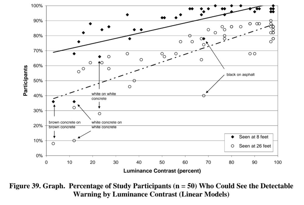
The goodness-of-fit for the linear models may be evaluated by the coefficient of determination, which for the 2.44 m (8 ft) distance is r2 = .56. For the 7.92 m (26 ft) distance, this value is r2 = .65. If the natural logarithm of luminance contrast is used to predict detection, the fit of the models improves substantially. In Figure 40, two logarithmic models have been fit to the data. The coefficients of determination (“r-square”) for these models are r2 = .76 for the 2.44 m (8 ft) data, and r2 = .73 for the 7.92 m (26 ft) data.
The model for predicting the percentage of participants seeing the detectable warning from a distance of 2.44 m (8-ft) (PS8) is:
PS8 = 16.18* Ln(percent contrast) + 25.77.
The model for predicting the percentage of participants seeing the detectable warning from a distance of 26 ft (PS26) is:
PS26 = 22.39* Ln(percent contrast) - 18.94
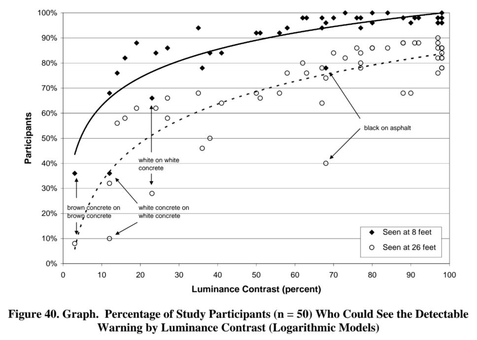
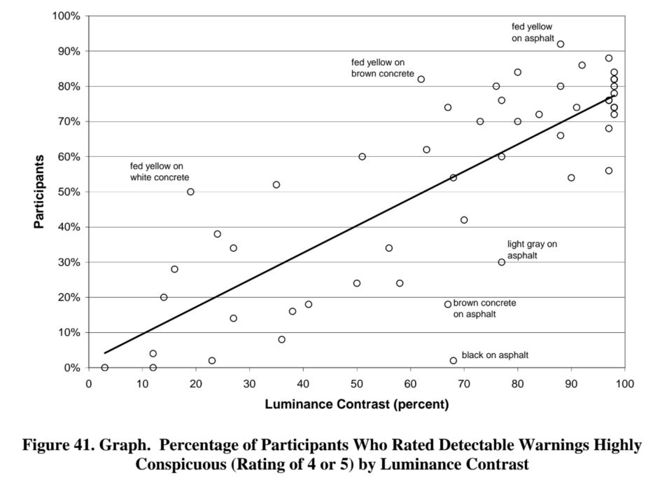
Figure 41 shows the percentage of participants who rated each combination of detectable warning and sidewalk highly conspicuous (rating of 4 or 5) as a function of luminance contrast. The figure shows a positive correlation (r = .80) between perceived conspicuity and luminance contrast. The figure also draws attention to some combinations of detectable warning and sidewalk that were rated either more or less conspicuous than others with similar luminance contrasts. The three most obvious “overachievers” include the federal yellow detectable warning on the white, brown, and asphalt sidewalks. On these sidewalks the federal yellow detectable warning received high conspicuity ratings from more participants than would be expected based on the contrast alone. The three most obvious “underachievers” include the asphalt sidewalk with the black, brown, and light gray detectable warnings. These three detectable warnings on the asphalt sidewalk were rated highly in conspicuity by fewer participants than would be expected based on their contrast.
The linear model used to fit the data for the percentage of participants giving high conspicuity ratings (PHC) is:
PHC = .77* (percent contrast) + 1.84.
This model has a coefficient of determination equal to r2 = .64. A logarithmic model (not shown here) did not fit these data as well as the linear model (r2 = .55), so for all subsequent analyses, contrast was used instead of log contrast to predict high conspicuity ratings.
2.9 Models to Predict Visual Detection and High Conspicuity Ratings
We conducted several regression analyses on the data shown in Figure 40 and Figure 41 to determine if adding additional parameters would substantially increase the correspondence between the models and the data. Contrast (or log contrast), reflectance of the detectable warning, reflectance of the sidewalk, and a binary parameter which encoded patterned versus single-color detectable warnings were used. A second binary parameter was used in the models to encode colored (bright red, orange-red, federal yellow, pale yellow) versus achromatic (black, white, gray) detectable warnings. For these analyses, the brown detectable warning was included with the achromatic set. Note that for the patterned detectable warnings, reflectance of the white area was used in all analyses requiring a value for detectable warning reflectance. In a second series of analyses (not shown here) the reflectance of the black area of the patterns was defined as the value for detectable warning reflectance, but this did not substantially affect the coefficients for the model parameters. The three best-fitting and simplest models are described below.
The model to predict the percent of participants who could see the detectable warning from 8-feet (PS8) is shown below. Its coefficient of determination is r2 = .82.
PS8 = 17* Ln(Contrast) + 20.3 + (7.3 if color is red or yellow).
The model to predict the percent of participants who could see the detectable warning from 26-feet (PS26) is shown below. Its coefficient of determination is r2 = .78.
PS26 = 23.4* Ln(Contrast) - 26 + (9.6 if color is red or yellow).
The model to predict the percent of participants who judged the detectable warning to have high conspicuity (PHC) is shown below. Its coefficient of determination is r2 = .82.
PHC = .806* (Contrast) + 19* RDW - 16.7 + (26.6 if color is red or yellow).
Where:
Contrast = percent luminance contrast (0-100)
RDW = reflectance (0-1.0) of the detectable warning (for patterns, reflectance of white areas was used).
2.10 Other Factors that May Predict Visual Detection and High Conspicuity Ratings
The study team conducted several logistic regression analyses of the trial-by-trial data to determine whether lighting conditions may have influenced visual detection and conspicuity of detectable warnings. We examined the effects of cloud cover per session and illuminance per trial along with reflectance of the detectable warning, reflectance of the side walk, the effect of using a single-color versus a patterned detectable warning, and the effect of using an achromatic (black, white, gray) versus a colored (bright red, orange-red, federal yellow, pale yellow) detectable warning.
For these analyses, the brown detectable warning was grouped with the achromatic set. Also note that, for the analyses described below, the reflectance of the white part of the patterned detectable warnings was defined as the detectable warning reflectance. In other analyses (not shown here) we defined the reflectance of the black area of the two-color detectable warnings as the detectable warning reflectance. The coefficients for nearly all model parameters were similar no matter which area was used to define reflectance for the two-color detectable warnings. The only exceptions were the parameter estimates for the pattern versus no pattern variables in the 7.92 m (26 ft) detection model and in the conspicuity model described below. For these two models, the pattern versus no-pattern parameter estimates were sensitive to the way that the reflectance was defined for two-color detectable warnings. All other parameter estimates, including the parameter for detectable warning reflectance, were not sensitive to the area (white or black) used to define reflectance of two-color detectable warnings.
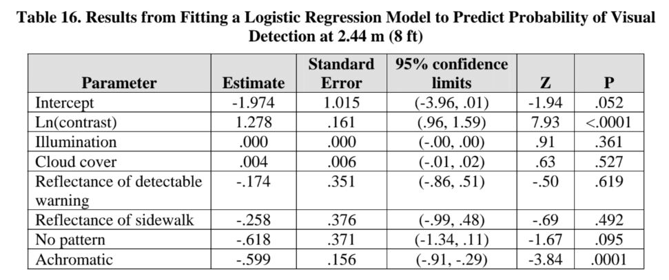
Three similar models were used to predict probability of seeing the detectable warning at 2.44 m (8 ft), the probability of seeing the detectable warning at 7.92 m (26 ft), and the probability of obtaining a high conspicuity rating (4 or 5). The data for these analyses were the outcomes of every trial on which a detectable warning was presented. Thus, the number of data points to be fit by each of the three logistic regression models was: 50 (participants) x 13 (detectable warnings) x 4 (sidewalks) = 2600. The logistic regression analyses were performed with SAS statistical software using the general linear model procedure (PROC GENMOD). The parameter estimation algorithm included an adjustment for repeated measures data clustered by participant.
The parameter estimates of the model for predicting the probability that a detectable warning would be seen from 2.44 m (8 ft) are shown in Table 16. It is clear from the parameter estimates that neither cloud cover nor illuminance help to predict whether a detectable warning would be seen from 2.44 m (8 ft) in this study. The logarithm of contrast, Ln(Contrast), and the parameter for achromatic versus colored have estimates significantly different from zero. Greater contrast increases the probability of detection at 2.44 m (8 ft) and using an achromatic detectable warning decreases the probability of detection as compared to the red or yellow detectable warnings. The negative estimates for the two reflectance parameters and for the no-pattern parameter are not statistically significant.
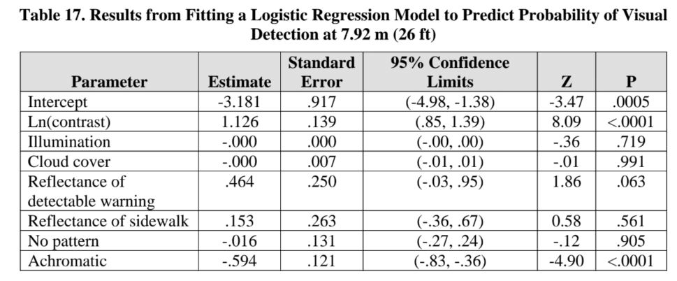
A similar regression model was used to predict the probability that a detectable warning would be seen from a distance of 7.92 m (26 ft). These results are shown in Table 17. In this model, illumination, cloud cover, and reflectance of the sidewalk do not help to predict whether the detectable warning will be seen. The statistically significant parameter estimate for the logarithm of contrast (p < .0001) indicates that higher contrast predicts a higher probability of visual detection at 7.92 m (26 ft). The achromatic parameter estimate is also statistically significant (p < .0001) indicating that having a colored (red or yellow) as opposed to an achromatic detectable warning increases the prob ability of detection from 7.92 m (26 ft). The positive estimate for reflectance of the detectable warning is not statistically significant.
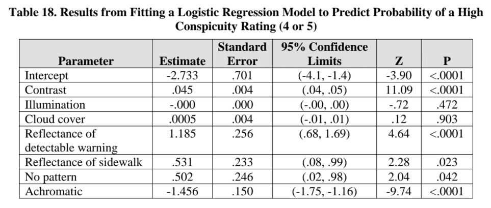
The results of a similar logistic regression model used to predict the probability of high conspicuity ratings are shown in Table 18. For this model, contrast was used rather than the natural logarithm of contrast. Consistent with the results of the two detection models described above, illumination and cloud cover do not help to predict conspicuity. However, several of the other parameter estimates are statistically significant.
The statistically significant model parameters include contrast (p < .0001), reflectance of the detectable warning (p < .0001) and no pattern (p < .05). According to the parameter estimates, higher contrast, higher reflectance of the detectable warning, higher reflectance of the sidewalk, and no pattern each increase the probability that the detectable warning will receive a high conspicuity rating. Having an achromatic detectable warning significantly decreases the probability of obtaining a high conspicuity rating as compared to the red and yellow detectable warnings (p < .0001). The effect of pattern versus no pattern in this model depends strongly on whether reflectance data for the white or for the black elements of the patterned detectable warnings were defined as detectable warning reflectance. All other parameter estimates were robust to this change.
2.11 Perceived Color of Detectable Warnings
The ability of people with visual impairments to correctly recognize the color of detectable warnings has important implications for both conspicuity and the potential for detectable warning color standardization. One possible reason to standardize detectable warning color is to have detectable warning color impart a specific meaning in the same way that the colors of various roadside signs have particular meanings. However, if color perception for pedestrians with visual impairments is not consistent across individuals or not stable among individuals or across lighting conditions, the “message” intended by the standardized color of a detectable warning may not be received by the intended recipients.
Participants were asked to describe the color of each detectable warning that they saw. These descriptions were made at a distance of 2.44 m (8 ft) from the detectable warning. Numerous color descriptions were given for each detectable warning and these descriptions often seemed to be influenced by the color of the sidewalk. For instance, the dark gray detectable warning was much more likely to be described as “black” on the white concrete sidewalk than it was on any other sidewalk. Presumably, this was because the high contrast provided by the white sidewalk made the detectable warning look darker by comparison. In most cases, participants provided color descriptions that were consistent with each other and with the visually unimpaired experimenters’ perceptions. However, for every detectable warning there were several unusual descriptions. The participants whose vision was most impaired were often the most likely to use color names not used by other participants. The complete set of color descriptions given by participants for each detectable warning and side walk combination is presented in Appendix F.
2.12 Comments from Participants
The experimenters did not solicit opinions or comments from participants regarding the detectable warnings outside of the data collection protocol. However, experimenters recorded comments whenever they were offered. Some participants commented frequently while others did not comment at all, so these comments should be considered individual opinions rather than group consensus. The complete list of comments is presented in Appendix G and major findings are summarized below.
The black-and-white stripes and the federal yellow detectable warnings received the most favorable comments. The black-and-white stripe detectable warning was often called “very attention-getting” and some participants called it their favorite detectable warning, but a few others noted that the pattern appears to have depth or looks like a metal grate. Some noted that the black stripes “disappear” when placed on the asphalt sidewalk. Many participants said that the federal yellow detectable warning was very likely to get their attention, but a few others were concerned that the contrast was insufficient on the white concrete sidewalk.
Some participants noted concerns about detectable warnings that might not be recognized as warnings or that might be mistaken for other things. Dark detectable warnings such as black, dark gray, and black with white border were sometimes thought to look like holes, asphalt patches, or shadows on the sidewalk. The light gray, dark gray, and white concrete detectable warnings were sometimes thought to look like concrete patches. The brown concrete and orange-red detectable warnings were some times thought to look like cardboard or rust.
The black-and-white patterned detectable warnings received mixed feedback on the white concrete sidewalk and the asphalt sidewalk. Although the internal contrast of these detectable warnings was typically sufficient to provide high visibility, some participants commented that the white sections of the detectable warnings blend into the white concrete sidewalk or did not help them to see the detectable warning. The same was said about the black sections of the detectable warnings on the asphalt sidewalk. These sentiments were most frequent with regard to detectable warnings whose borders were similar in reflectance to the sidewalk (e.g., white border/white concrete sidewalk; black border/black asphalt sidewalk). The black–and-white stripe pattern sometimes looked like a metal grate to two participants.
User Comments/Questions
Add Comment/Question